Fig 1: Road Example
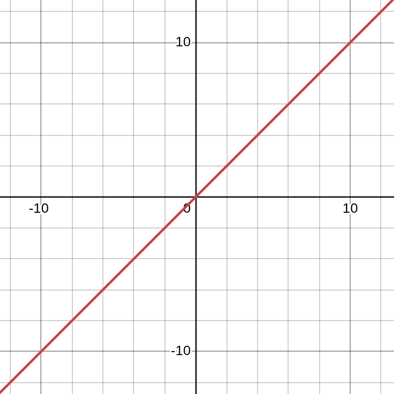
Fig 2: Graph illustration
Before we can delve any further into machine learning / neural networks work, we need to understand the mathematical (calculus) topic of derivatives. This is a core aspect present in almost all standard neural networks and entails the magic sauce that enables neural networks to learn.
P.S. If you are well versed with derivatives, feel free to skip this section completely.
Important note: The topic of derivatives is huge in mathematics/calculus, and we obviously cannot cover it in great detail here (that will be a blog series on its own, and move away from the core objective of this blog series). What we cover here are the main key concepts you should know for machine learning. If the explanation seems inadequate, we would encourage you to go read or watch a more detailed video on this topic. Having said that, it is important you understand derivatives, as this is core to understanding neural networks from first principles.
What is a derivative?
Succinctly, you can say a derivative is a measure of the rate of change for a given function. For some, this might make sense, and for others, not so much. To help illustrate this, I will use a simple example.
Imagine you are taking a stroll in your neighborhood. You then decide to take a turn, and behold, this is an uphill road that has an incline of 45 degrees all the way to the top. Diagrammatically, you represent this as
|
|
|
|
Fig 1: Road Example |
Fig 2: Graph illustration |
If you plot a graph of this, you can easily see that for each 1m you move on the
ground level, your altitude increases by 1m. In
essence, you can say there is a 1-to-1 relationship between the distance you move on the ground and the
effect it has on your altitude. This ratio  — the rate of change — is what we call the
derivative of the relationship between moving on the ground floor and its impact on altitude (p.s., we are
using point 0 as a starting point, but we could have used any other point).
— the rate of change — is what we call the
derivative of the relationship between moving on the ground floor and its impact on altitude (p.s., we are
using point 0 as a starting point, but we could have used any other point).
Formulaically what we are saying is  , or more graphically
  , and
since our derivative in this case is 1, we end up with
, and
since our derivative in this case is 1, we end up with  as the formula.
What if the road was more inclined? For instance, for every 1m on the ground, we move 2m in altitude. In
this case, the derivative would be  . Therefore, the
formula would be
. Therefore, the
formula would be  .
.
From this, we can see a pattern emerging, that is, the derivative (denoted
 ) of a straight line is the constant (
 ) accompanying
  is the equation
  .
.
Key Point: In fact, they are rules for working out the
derivatives of any equation. For a case like the above (), you multiple the power of the element (which is 1) by the constant ( and the you reduce the power of the element by one, making it 1. I.e

Derivate at a point / for curved graphs
In this road example above, we kept it quite simple by making the road straight. Let's however, imagine that the road is ‘curved’ (p.s. the road example is not the best example in this case, but bear with me).
In this case, our derivative cannot be constant, as the rate of change/derivative changes depending on where you are on that road. To illustrate it better: imagine letting a ball descend from the top. As the ball descends down the road, its rate of change (i.e., the ratio between distance traveled on the ground and altitude) is different at each point.
It is for this reason why in curved graphs we talk about the rate of
change/derivative at a point. Mathematically, we would say when the degree of a polynomial is greater than 1
(i.e  ), the derivative (for ), will be a function that gives a derivative at a point.
Using the rule cover above, the derivative of  will be
  . Hence, the rate of change at
 , be 2.
Chain rule of derivates:
The last thing we need to note when it comes to derivatives (before seeing their use in neural networks) is the chain rule. This states that if you have a function

And another one

To get the derivative  you
you
 as a variable in the
  function and get the derivative of that - which will be
  , then multiple it with the derivative of - which will be 2
P.S. As already mentioned, if this is confusing (or not as clear), we encourage you to take some time out to read more on this. It does become clearer the more you read on it.
What does this have to do the machine learning/neural networks
To explain this, let's go back to the straight line road example with the
equation . IImagine I say we want to know the ground distance moved ( when the altitude (
 is 5. Simple: we want to solve for
  .
.
Now, from basic algebra, you could easily solve this by dividing by 2 on both sides. However, from a machine learning perspective, it should be able to learn how to solve this itself (i.e., not follow predetermined rules). Therefore, the question is: how would machine learning go about solving this?
Firstly, we define a cost
function, which is a measure of how far off any answer is from the expected
answer. In this case, we can make it C =  (which is
  ). Since we now have this cost function, our aim is to make this
approach 0, which in essence means we want
). Since we now have this cost function, our aim is to make this
approach 0, which in essence means we want

Secondly, in this equation above, we know that the derivative of the cost function C = with respect to is 2. Knowing this, we can deduce that if we move forward along this
derivative/gradient, our new value for and
and  will increase, and conversely if we
move backwards the value decreases.
will increase, and conversely if we
move backwards the value decreases.
Now with this, we can derive a strategy where we:
, and then move a small distance  (known in machine learning as the learning
rate) 'along' this gradient., and conversely, get a new value for
(known in machine learning as the learning
rate) 'along' this gradient., and conversely, get a new value for 
 when = 5.
Illustratively, let's say we start off with  . In this
case, our cost is 5 (i.e.,
. In this
case, our cost is 5 (i.e.,  ). Since this is more than zero, we want to
move backward along our gradient to get a new by a distance of , which we can make 0.25. Therefore,
). Since this is more than zero, we want to
move backward along our gradient to get a new by a distance of , which we can make 0.25. Therefore,
 =
= 
= 
= 
We can then check this again until we arrive at the place where our cost approaches zero. This is illustrated in the table below.
|
|
Current x |
Cost value |
|
Derivate x Learning rate |
New x |
|
1st Run |
5 |
5 |
|
0.5 |
4.5 |
|
2nd Run |
4.5 |
4 |
|
0.5 |
4 |
|
3rd Run |
4 |
3 |
|
0.5 |
3.5 |
|
4th Run |
3.5 |
2 |
|
0.5 |
3 |
|
6th Run |
3 |
1 |
|
0.5 |
2.5 |
|
7th Run |
2.5 |
0 |
|
|
|
Now, of course, this above is a
well-curated example in which the learning rate ( and the selected values, allow you to arrive at a precise
answer (i.e., not overshooting) within a reasonable time/learning steps (7 steps). However in most cases, this would not be the case - for instance, imagine what would happen if
our learning rate was 0.7, etc.?
and the selected values, allow you to arrive at a precise
answer (i.e., not overshooting) within a reasonable time/learning steps (7 steps). However in most cases, this would not be the case - for instance, imagine what would happen if
our learning rate was 0.7, etc.?
To handle this, we need to think of a different cost function that can handle scenarios like this. One common approach in neural networks is to square the difference between the current value and the expected value (this is known as Mean Squared Error or MSE). For instance, using our function above, this new cost function will be:

This still works to determine as when you approach 0, whether the function is squared or not, it approaches the same
value (i.e.,  ). However,
there are now some advantages:
). However,
there are now some advantages:
 is itself a function of (i.e
  ) , we don’t have to worry about what direction to move as the
value will give us that
information. itself.
) , we don’t have to worry about what direction to move as the
value will give us that
information. itself.To better illustrate the above points, let's mimic the learning process in the
table below. Note in this case, we will make our
learning rate  , and our
initial .
, and our
initial .
The update rule is:
=
= 
= 3
|
|
Current x |
Cost value |
|
Derivate x Learning rate |
New x |
|
1st Run |
5 |
25 |
|
2 |
3 |
|
2nd Run |
3 |
1 |
|
0.4 |
2.6 |
|
3rd Run |
2.6 |
0.04 |
|
0.08 |
2.52 |
|
4th Run |
2.52 |
0.0016 |
|
0.016 |
2.504 |
|
|
|
|
|
|
|
|
|
|
|
|
|
|
As you can see from the above, the benefit of using the Mean Squared Error function is that
you choose, it will always move
towards 0—it will always descend toward the lowest point, hence the process is commonly known in
machine learning as gradient
descent.Notes on Learning Rate and Overshooting
And that's about it!
Key Point: At a rudimentary level, this is what neural networks are doing, albeit with more chained functions and other nuances. In essence, neural networks involve:
Quick caveat: This approach, which is rooted in derivatives, follows a family of algorithms that use gradient descent as their main/root technique. From an academic perspective, there are other research approaches that try to do away with derivatives. However, they are in the realm of academic research. In fact, standard and well-known neural network libraries like PyTorch only offer algorithms that are rooted in gradient descent.