Let's imagine we want to create a machine learning algorithm that determines whether a certain property is worth investing in or not.
In a real-world use case, you would gather as much labeled data as possible—that is, data on previously sold properties (including as many features as possible, such as price, location, aesthetic beauty, age, surrounding amenities, etc.) and how they performed. With that data, you would create your neural network, using the (normalized/standardized) features as inputs and comparing the output with the labeled data.
Since we do not have that data here (and our objective is to learn how they work, as opposed to creating a real neural network), we are going to mimic a simplified version of this data. In our case, we are going to imagine our property only has three features: price, surrounding amenities (score out of 10), and aesthetic beauty (score out of 10).
If our property price is below R700 000, with an aesthetic score above 7, and a surrounding amenities score above 8, we are going to mark this as a good investment.
To create this sample labeled data, we can use the Python script found here. This script will create a CSV file of the data and an additional JSON file with the corresponding standardized data (which we will actually train our model on). Examples of this data are highlighted below:
|
price |
amenities_score |
aesthetic_score |
is_good_investment |
|
1879663 |
9 |
10 |
0 |
|
297277 |
10 |
8 |
1 |
|
635708 |
10 |
4 |
0 |
|
584470 |
9 |
9 |
1 |
{
"input": [
[
2.6699167069379803,
0.24143092618135178,
0.8400655569795001
],
[
-0.6956048300055256,
0.6555491529075125,
-0.06566550175850519
],
...
"output": [
[
0
],
[
1
]
....
}
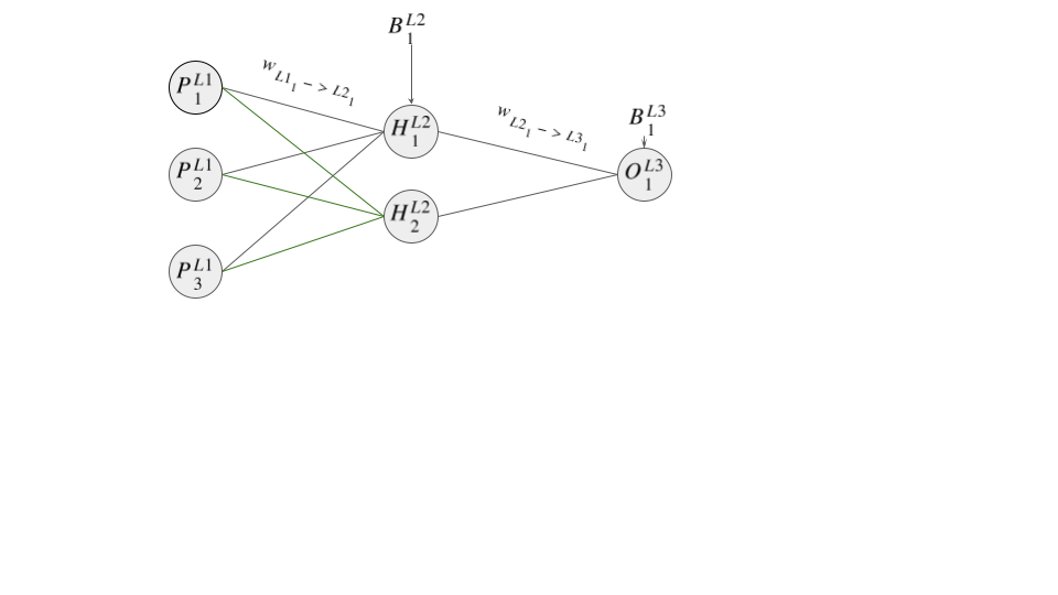
Now that we have our mimic data, we are going to create our neural network with one hidden layer. Diagrammatically, this can be displayed as
Note:
Strictly speaking, since the data we created is linearly separable, we could omit a hidden layer. However, in most cases, data requiring a neural network is not linearly separable. For example, imagine a scenario with a more complex decision boundary, such as if the property price is below R700 000, with an aesthetic score above 7, and a surrounding amenities score above 8, OR if the price is below R350 000, with a surrounding amenities score above 8, and an aesthetic score above 5. This more complex data would require a hidden layer to effectively capture these characteristics or patterns. For the sake of completeness, we are including a hidden layer in this example.
As already highlighted, the first step in the neural network learning process is forward propagation. This starts off at the input layer and propagates forward till the output layer.
In the first layer, for the nodes  ,
,
 , and
, and  get the values
= 
=
= 
Based on our previous highlighted formula (under activating function), the values of the hidden layer will be
 =
= 
 =
= 
Even though these values are correct, remember we need to take them through our activation
function (  ) so as to get the activation value (
 ). Therefore
 =
= 
 =
= 
Our output layer takes the activation values of the previous layer, and does the same operation as before to get the final value. That is
 =
= 
And again, we need to put it through our activation function
 =
= 
And that's it. For a given input, we have a predicted value, completing the forward propagation cycle.
Now that we have our output/predicated value, we can now work out the cost of this run through (using the MeanSquare Error cost formula). For that we get
 = (
= (
With this you would then check if the cost value is close to zero. If not, you would move onto adjusting the weights and biases via
backpropagation (with the caveat of mini-batching - see below), and repeat the cycle.
The walkthrough/example above was designed to explain forward propagation as simply as possible. There are, however, some small caveats you need to be aware of for real use cases.
Cost of Multiple Nodes
In the preceding example, the network featured a single output node, resulting in a cost
calculated as . However, most scenarios involve multiple
output nodes. In such cases, the overall cost is typically determined by averaging the
individual costs. Using Mean Squared Error (MSE), the formula is:
. However, most scenarios involve multiple
output nodes. In such cases, the overall cost is typically determined by averaging the
individual costs. Using Mean Squared Error (MSE), the formula is:

Mini Batching
As will be seen in the next entry, backpropagation is the more computationally intensive part of machine learning. Because of this, performing it after every forward propagation would be quite expensive (considering that many neural networks may have thousands of nodes).
It is for this reason that it is standard practice in machine learning to batch forward propagations, and then after a certain number, perform the backpropagation, using 'average' values where applicable.
Vector/matrix operations
The formulas above show how each node was updated. In practice, though (and in most explanations of machine learning), this updating happens via vector/matrix operations. The main reason for this is speed, as iterating through each node would be computationally inefficient. It also has the benefit of making most of the formulas more compact. For instance, for layer 2, we could just say

Where  is a vector of
the layer 2 nodes (and conversely
is a vector of
the layer 2 nodes (and conversely  at layer 1),
and
at layer 1),
and  is the vector of biases at layer 2,
 the weight matrix between the 2
layers,
the weight matrix between the 2
layers,
Although this is the primary way neural network operations occur, for those not well-versed with vector/matrix operations, this can get quite confusing—blurring the more straightforward underlying logic of neural networks. It is for this reason that, where possible, we choose the more verbose/'inefficient' form.
Do note: In our accompanying codebase, we aim to use different implementation approaches (with the same interface) so you can try to connect what happens (i.e., between vanilla Python, with NumPy—vector/matrix manipulation, PyTorch, and TensorFlow).